Structure generation

Directory: "examples/graphene/01_generate_monolayer":

In main input for QNANO is a file containing the positions of all atoms in the structure. Here, we create 3 different graphene samples:

8x8 unit cells of graphene
a hexagonal flake with armchair edges (size: 8 hexagonal rings per side)
a hexagonal flake with zigzag edges (size: 8 hexagonal rings per side)
a triangular flake with zigzag edges (size: 5 hexagonal rings per side)

To run the example, go to an empty directory and call:

$QNANO_DIR/examples/graphene/01_generate_monolayer/run_example.sh

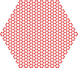
This command will have created three postscript files "positions_Nx8_Ny8.ps", "positions_armchair_hex8.ps", "positions_zigzag_hex8.ps", and "positions_tri5.ps" that can be opened with any vector graphics reader (e.g. evince on Linux).

The result is shown below:

positions_Nx8_Ny8.ps:

positions_armchair_hex8.ps:

positions_zigzag_hex8.ps:

positions_tri5.ps:

This script invokes command for generating the structure and for generating the postscript file:

The command

$QNANO_DIR/bin/generate -materialfile $QNANO_DIR/resources/graphene.dat \
-Nx 8 -Ny 8 -outfile positions_Nx8_Ny8.dat

generates a positions file with a name specified by the option "outfile" using the material defined by the material file "$QNANO_DIR/resources/graphene.dat". This materialfile contains information about the lattice constants and a reference to the lattice file (which is in this case "$QNANO_DIR/resources/hex2D_vdW.dat").

The options "-Nx 8 -Ny 8" tell the tool to create a lattice with 8 unit cells in x- and y-directions. For the hexagons, we can use instead the options "-cut_hexagon_armchair 8" and "-cut_hexagon_zigzag 8".

As arbitrary shapes of structures can be arbitrarily complicated, we leave the generation of postions files for other scenarios to the user. To this end, we want to clarify the format of the position file. For example, the first 12 lines of the file "positions_Nx8_Ny8.dat" are:

<materials>
 material   1   graphene
</materials>

number_of_atoms 128

atom_data
      0 0 0 6
      0.071000014 0.12297561 0 6
      0.213 0.12297561 0 6
      0.28400001 0.24595121 0 6
      0.426 0.24595121 0 6
...

The block "<materials>" contains information about the material. In this case it is "graphene" and the code will look for a file "graphene.dat" in the specified resources directory. Then, the total number of atoms in the structure is specified. After "atom_data" the actual block of atoms follows: Each line corresponds to one atom, the first 3 numbers are x, y and z coordinates in nm, the last number is an identifier of the element. We typically use the number in the periodic table, i.e. 6 for Carbon.

In the next step, we display the generated stuctures via postscript files. The tool for this is "QNANO2ps" and can be invoke like

$QNANO_DIR/bin/QNANO2ps -positions positions_Nx8_Ny8.dat -outfile positions_Nx8_Ny8.ps

where the option "-positions" specifies the positions file of the structure to be displayed and "-outfile" sets the name of the generated postscript file.

However, we do provides some basic cutting features. As an example, we explain the steps involved in cutting the zigzag triangle

N=5
$QNANO_DIR/bin/generate -materialfile $QNANO_DIR/resources/graphene.dat \
-Nx $(($N+2)) -Ny $(($N+2)) -outfile positions_tri${N}.dat \
-cut_plane_through_LU -1 0 0 $(echo $N-0.01|bc) 0 0 \
-cut_plane_through_LU_LU 0.666667 -0.333333 0  $(echo $N+1.01|bc) 0 0 \
-cut_plane_through_LU_LU -0.333333  0.666667 0   0 $(echo $N+0.01|bc) 0 \
-cut_plane_through_LU 0 -1 0 0 $(echo $N-0.01|bc) 0  \
-cut_plane_through_LU 1 0 0  $(echo 2*$N+0.99|bc) 0 0

where N controls the size, i.e. the number of hexagonal rings per side of the triangle.

The tool first generates a sample composed of 7x7 unit cells, which will be large enought to contain a part from which we can cut out the triangle. Subsequently the sample is cut using planes. A plane can be specified by its Hesse normal form, i.e. a vector perpendicular to the plane and the shortest distance to the origin (option "cut_plane", not used here). Here, we use the alternative of setting the shortest distance to zero, but specifying the origin as a point explicitly. "cut_plane_through" therefore has 6 arguments, the first three are the direction vector (perpendicular to the plane) and the last three are center coordinates. By default, the origin set to the point from which the underlying unit cells are created (here: the leftmost atom in the structure before cutting) and the coordinates are given in units of nm. "cut_plane_through_LU" uses "lattice units" for the origin, i.e. the coefficients will be multiplied with the respective lattice vectors, while the direction vector is still provided in cartesian coordinates. The option "cut_plane_through_LU_LU" uses lattice units for both, the origin and the direction vector.

The individual steps required for cutting are illustrated below: