Prestrained plates
Prestrained thin materials develop internal stresses, deform out of plane, and exhibit nontrivial 3D shapes even without external forces. Chief examples exhibiting such phenomena are nematic glasses, natural growth of soft tissues or manufactured polymer gels. After reduction from 3D to 2D, denoting by $\Omega\subset\mathbb{R}^2$ the midplane of the plate, the model consists in minimizing the bending energy $$ E(\mathbf{y}) = \frac{\mu}{12}\int_{\Omega}\big|g^{-\frac{1}{2}} \, {\rm II}(\mathbf{y}) \, g^{-\frac{1}{2}}\big|^2+\frac{\lambda}{2\mu+\lambda}{\rm tr}\big(g^{-\frac{1}{2}}\, {\rm II}(\mathbf{y}) \, g^{-\frac{1}{2}} \big)^2 $$ under the constraint that $$\nabla\mathbf{y}^T\nabla\mathbf{y}=g \quad \mbox{a.e. in } \Omega.$$ Here, ${\rm II}(\mathbf{y})$ denote the second fundamental form of the deformed plate $\mathbf{y}(\Omega)$, $\mu$ and $\lambda$ are the Lamé coefficients, and $g$ is the given (symmetric positive definite) target metric. The second fundamental form can actually be replaced by the Hessian of the deformation without affecting the minimizers. In the proposed numerical method, an LDG approach is used for the discretization, where the Hessian is replaced by a so-called discrete Hessian consisting of the broken Hessian and the liftings of jump terms, and an $H^2$ gradient flow is used for the energy minimization.
Manufactured gel discs
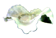
A laboratory experiment, where prestrained discs made of NIPA gel with various monomer concentrations are manufactured, is presented in [3]. Considering a similar metric, see [3, Section 5.5] for details, the proposed numerical method produces deformations that are comparable to the experimental ones.
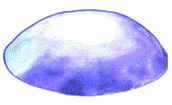
Laboratory manufactured disc gels using an elliptic prestrained metric $g$ along with the approximate equilibrium shape.
Laboratory manufactured disc gels using a hyperbolic prestrained metric $g$ along with the approximate equilibrium shape.
Metric with positive Gaussian curvature
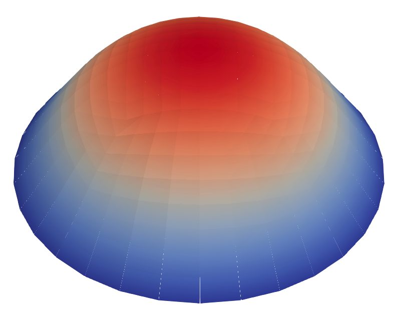
In this example, we consider the bending of the unit disc when a metric with positive Gaussian curvature is prescribed, namely $$ g = \nabla\mathbf{y}^T\nabla\mathbf{y} \qquad \mbox{with} \qquad \mathbf{y}(x_1,x_2)=\left(x_1,x_2,\sqrt{0.2}\sin\Big(\frac{\pi}{2}\big(1-\sqrt{x_1^2+x_2^2}\big)\Big)\right)^T, $$ where $\mathbf{y}$ corresponds to the parametrization of a bubble. We do not impose any boundary conditions (free boundary case). Before running the gradient flow algorithm, a pre-processing step is used to get an initial deformation with a prestrain defect below 0.1.
Evolution of the deformation throughout the gradient flow for the unit disc with a positive Gaussian curvature metric.
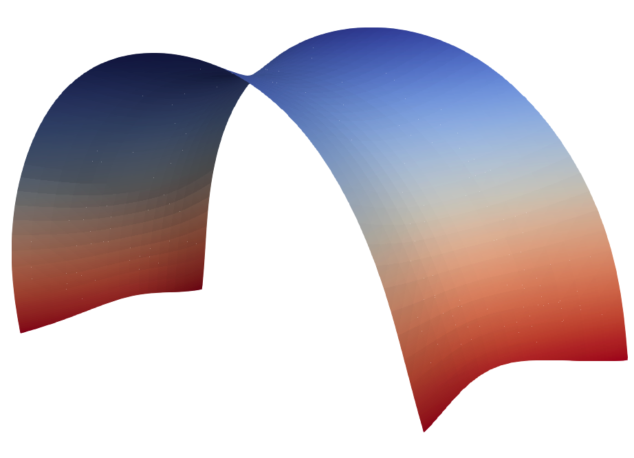
Metric with negative Gaussian curvature
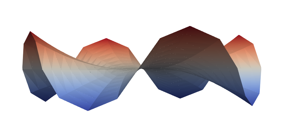
We use the same setting as in the previous example but with the metric $$ g(x_1,x_2) = \begin{bmatrix} 1+x_2^2 & x_1x_2 \\ x_1x_2 & 1+x_1^2 \end{bmatrix} $$ which has a negative Gaussian curvature and is achieved by the deformation $\mathbf{y}(x_1,x_2)=(x_1,x_2,x_1x_2)^T$ corresponding to a hyperbolic paraboloid.
Evolution of the deformation throughout the gradient flow for the unit disc with a negative Gaussian curvature metric.
Metric corresponding to a catenoid/helicoid
Here, $\Omega\subset\mathbb{R}^2$ is a rectangular domain and we prescribe the metric $$ g(x_1,x_2) = \begin{bmatrix} \cosh(x_2)^2 & 0 \\ 0 & \cosh(x_2)^2 \end{bmatrix}. $$ The deformations $$ \mathbf{y}^{\alpha}(x_1,x_2)=\cos(\alpha) \begin{bmatrix} \sinh(x_2)\sin(x_1) \\ -\sinh(x_2)\cos(x_1) \\ x_1 \end{bmatrix} + \sin(\alpha) \begin{bmatrix} \cosh(x_2)\cos(x_1) \\ \cosh(x_2)\sin(x_1) \\ x_2 \end{bmatrix} $$ are all compatible with the metric and all give the same energy. The case $\alpha=0$ corresponds to an helicoid while $\alpha=\pi/2$ represents a catenoid.


Final configurations for the free boundary case with different initial deformations: from left to right, the prestrain defect of the initial deformation is about 2.6, 1.4 and 0.9. The smaller the defect, the closer the final shape is to be a closed catenoid.
Evolution of the deformation throughout the gradient flow. Left: free boundary case; right: view from the side and from the top when boundary conditions for $\nabla\mathbf{y}$ and $\mathbf{y}$ are prescribed on the bottom side of the rectangle.
| [1] | A. Bonito, D. Guignard, R.H. Nochetto, and S. Yang. LDG approximation of large deformations of prestrained plates. Submitted (ArXiv preprint). |
| [2] | A. Bonito, D. Guignard, R.H. Nochetto, and S. Yang. Numerical analysis of the LDG method for deformation of prestrained plates. Submitted |
| (ArXiv preprint). | |
| [3] | E. Sharon and E. Efrati. The mechanics of non-euclidean plates. Soft Matter 6(2):5693-5704, 2010. |
Other projects
under construction...